Resampling
Resampling is a technique applied in various image processing tasks, most prominently scaling/resizing, but also shifting and rotation.
Resizing
The most common class of resampling algorithms used for resizing are the convolution-based resamplers. As the name suggests, these work by convolving the image with a filter function. These filter functions, also known as kernels, are what the terms Bilinear/Bicubic/Lanczos/etc. generally refer to. The ImageWorsener documentation features a great visual explanation of how this process works in detail. It is strongly recommended to read it. If you wish to explore the mathematics behind the design of these filters, the Sampling and Reconstruction chapter of Physically Based Rendering is one of the best places for a layman to start.
Filters
All resampling kernels behave slightly differently and generate artifacts of differing kinds and severity.
It should be noted that there is no “objectively best” resampling filter, so it is largely a matter of personal preference. There are no hard and fast rules about which resampler performs best for any given type of content, so it’s best to test them yourself.
A short overview of the most common filters follows. For a much more extensive explanation of the different filters, including details on the exact algorithms, see ImageMagick’s guide.
Additionally, ResampleHQ's documentation features an excellent visual comparison of common filter kernels; a back-up is available here.
Box filter / Nearest Neighbor
When upscaling, the Box filter will behave just like Nearest Neighbor (NN) interpolation, that is, it will just pick the closest pixel in the input image for every output pixel. This results in the source pixel grid being magnified without any smoothing or merging of adjacent pixels, providing a faithful representation of the original pixel grid. This is very useful when inspecting an image up close to examine the pixel structure, or when enlarging pixel art, but not suitable for regular content due to the jagged lines and deformed details it causes.
When downscaling, the Box filter behaves differently to NN—which continues to just pick the closest pixel and be done with it—in that it instead merges adjacent pixels together. (This is because generally, filter kernels are widened in proportion to the scaling factor when downscaling, which, in effect, applies a low-pass filter that serves to prevent aliasing.) Unlike most other filters, however, it averages them evenly instead of giving the central ones more weight. (For example, reducing a 10 pixel row to 5 pixels will average every pixel pair.) This, again, can be a useful property in specific cases, but is not generally desirable.
The Box filter is available in VapourSynth
in the fmtconv plug-in:
clip = core.fmtc.resample(src, w, h, kernel="box")
Nearest Neighbor interpolation is part of the built-in resize plug-in:
clip = core.resize.Point(src, w, h)
Most script editors including VSEdit feature NN scaling in the preview; it is recommended to use it over Bilinear when making filtering decisions.
Bilinear / Triangle
Bilinear, also known as Triangle due to its graph’s shape, is one of the most common algorithms in widespread use because of its simplicity and speed. However, it generally creates all sorts of nasty artifacts and is inferior in quality to most other filters. The only advantage it offers is speed, so don’t use it unless you’re sure you have to.
VapourSynth example:
clip = core.resize.Bilinear(src, w, h)
Mitchell-Netravali / Bicubic
The Mitchell-Netravali filter, also known as Bicubic, is one of the most popular resampling algorithms, and the default for many image processing programs, because it is usually considered a good neutral default.
It takes two parameters, B and C,
which can be used to tweak the filter’s behavior.
For upscaling, it is recommended to use values that satisfy the equation
b + 2c = 1.
The graph below outlines the various kinds of artifacts different B-C-configurations produce.

Roughly speaking, raising B will cause blurring and raising C will cause ringing.
Mitchell-Netravali generalizes all smoothly fitting (continuous first derivative) piece-wise cubic filters, so any of them can be expressed with the appropriate parameters. Below you can find a list of common cubic filters and their corresponding parameters in Mitchell-Netravali.
- B-Spline – b=1, c=0
- Hermite – b=0, c=0
- Mitchell-Netravali – b=⅓, c=⅓ (sometimes referred to as just “Mitchell”)
- Catmull-Rom – b=0, c=0.5
- Sharp Bicubic – b=0, c=1
Hermite is often considered one of the best choices for downscaling, as it produces only minimal artifacts, at the cost of slight blurriness.
VapourSynth example:
# 'filter_param_a' and 'filter_param_b' refer to B and C, respectively
clip = core.resize.Bicubic(src, w, h, filter_param_a=0, filter_param_b=0.5)
Lanczos
Lanczos is generally considered a very high-quality resampler for upscaling, especially its EWA version.
It is usually slightly sharper than Mitchell (Bicubic b=c=⅓), but might produce slightly more ringing.
Lanczos takes an additional parameter that controls the filter’s number of lobes, or taps. Increasing the number of lobes improves sharpness at the cost of increased ringing. You might occasionally see the tap count appended to the filter name to clarify the exact filter used, e.g. Lanczos2 for 2 taps.
For downscaling, higher tap counts might help in suppressing Moiré effects.
# 'filter_param_a' specifies the tap count
clip = core.resize.Lanczos(src, w, h, filter_param_a=2)
Spline
Spline is another high-quality resizer.
Spline, like Lanczos,
can be fine-tuned by configuring its number of lobes.
Unlike Lanczos,
however,
Splines with different tap counts are usually split
into separate functions,
with (tap_count∗2)^2 appended to their name,
e.g. Spline36 for 3 taps, Spline64 for 4, etc.
(This number represents the total amount of input pixels
involved in the calculation of any given output pixel.)
Spline36 is a very popular choice for downscaling, since it is fairly artifact-free yet decently sharp. For upscaling, it looks similar to Lanczos3, though arguably slightly less artifacted.
VS example:
clip = core.resize.Spline36(src, w, h)
Higher tap counts can be used via fmtconv:
clip = core.fmtc.resample(src, w, h, kernel="spline", taps=6) # equivalent to Spline144
Gauss
The Gaussian filter is very special in that its Fourier transform1 is another Gaussian whose width is inversely proportional to the spatial function’s. This can be harnessed to remove and amplify high frequencies in a very controllable way. Widening the filter, for example, will confine the output to small frequencies (blurrier), whereas squashing it will amplify higher frequencies (more aliasing).
In practice, though, the Gaussian filter isn’t all too useful for regular resizing. However, it can be used to accurately emulate a Gaussian blur (when used without resizing) in VapourSynth.
For example:
blurred = core.fmtc.resample(src, kernel="gauss", fh=-1, fv=-1, a1=1)
fh=-1, fv=-1 forces the processing
when no resizing is performed.
a1 controls the blurring:
the higher,
the sharper the image.
Interpolation filters
Some sources will categorize filters as either interpolation filters or non-interpolation filters.
Interpolation filters are those that when applied “in-place”, i.e. at the location of the input samples, don’t alter the sample value. Therefore, they only interpolate “missing” values, leaving the input samples untouched.
This is true for filters that evaluate to 0 at all integer positions except 0 or whose support is <= 1. Examples include: (Windowed) Sinc filters, such as Lanczos, Bicubic with B=0, e.g. Hermite and Catmull-Rom, and Triangle/Bilinear.
This can be a beneficial property in some cases, for example the No-Op case. No-Op means that no scaling, shifting or similar is performed, that is, the input is resampled at exactly the same positions. In this case, an interpolation filter will return the input image untouched, whereas other filters will slightly alter it.
Another, more practical, case where this property is useful is when shifting an image by full pixel widths (integers), again because input pixel values aren’t changed but just relocated.
Two-dimensional resampling
There are two different ways to go about resampling in two dimensions.
Tensor resampling (orthogonal, 2-pass, separated)
The image is resampled in two separate passes: First it is resampled horizontally, then vertically. This allows images to be treated 1-dimensionally since each pixel row/column can be resampled separately. The main advantage of this method is that it's extremely fast, which is why it’s the much more common one; generally, unless indicated otherwise, this is what is used.
Elliptical Weighted Averaging ("EWA", cylindrical, polar, circular)
All input samples whose Euclidean distance to the pixel is within the filter’s radius contribute to its value. The Euclidean distance is passed to the filter kernel. This is a lot more costly than tensor resampling in terms of runtime.
Scaling in modified colorspaces
The colorspace used when resampling can significantly impact the output’s subjective quality.
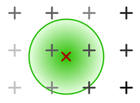
Downscaling in linear light
Downscaling in gamma-corrected light instead of linear light can sometimes noticeably dim the image. To see why this happens, consider this gradient:

It should be apparent that the brightness doesn’t scale linearly with the pixel values. This is because most digital video uses gamma-transformed pixel values in order to compress more perceptually distinct color shades into 8 bit. This causes the encoded pixel values to deviate from their expected brightness, e.g. a grey pixel has value 187 instead of 127 in sRGB. This poses a problem when merging and interpolating colors, because the average pixel value of two colors no longer corresponds to their average perceived brightness. For example, if you wanted to merge black and white (0 and 255), you would expect to get grey, but since grey actually has a value of ~187, the output pixel would turn out substantially darker, if you were you to naively average the pixel values.
To calculate the correct values, the gamma transform needs to be reversed before scaling and re-applied afterwards.
The dimming effect of scaling in gamma-corrected light is usually only noticeable in dense color patterns, e.g. small black text on a white background, stars in the night sky, etc, and much less so in blurrier areas.
See this comparison for a particularly extreme example of linear vs gamma downscaling.
However, this doesn’t necessarily mean downscaling in linear light is always the right choice, since it noticeably accentuates dark halos introduced by scaling. Thus, it may be wise to scale in gamma light when using a resizer prone to overshooting, like high-lobe Lanczos. Besides, the dimming may even be desirable in some cases like black text on white paper, because it preserves legibility.
If you choose to downscale in linear light, make sure to use a sufficiently high bitdepth so as to not introduce banding.
Example code for resizing in linear RGB light:
linear = core.resize.Bicubic(src, format=vs.RGBS, transfer_in_s="709", transfer_s="linear", matrix_in_s="709")
scaled_linear = core.resize.Bicubic(linear, 640, 360)
scaled_gamma = core.resize.Bicubic(scaled_linear, format=src.format, transfer_s="709", transfer_in_s="linear", matrix_s="709")
Note that the matrix_s and matrix_in_s arguments
are only necessary when src is YUV;
otherwise, they should be omitted.
Upscaling in sigmoidized light
In order to attenuate both dark and white halos introduced by upscaling, you can resize through a sigmoidized colorspace.
This means converting the linear RGB version of an image to a custom colorspace with an S-shaped intensity curve before scaling and converting it back afterwards. What this does, essentially, is decrease the image’s contrast by pushing extreme values of both dark and bright towards the middle.
Quoting Nicholas Robidoux from ImageMagick:
You may decrease halos and increase perceptual sharpness by increasing the sigmoidal contrast (up to 11.5, say).
Higher contrasts are especially recommended with greyscale images (even "false RGB greyscale" that have three proportional color channels).
The downside of sigmoidization is that it sometimes produces "color bleed" artefacts that look a bit like cheap flexographic ("gummidruck") printing or chromatic aberration.
In addition, sigmoidization's "fattening" of extreme light and dark values may not work for your image content.
If such artefacts are obvious, push the contrast value down from 7.5 (to 5, for example, or even lower).
Setting the contrast to 0 is equivalent to enlarging through linear RGB.
(Robidoux, 2012)2
Example code for VS:
import havsfunc as hf
linear = core.resize.Bicubic(src, format=vs.RGBS, transfer_in_s="709", transfer_s="linear", matrix_in_s="709")
sigmoidized = hf.SigmoidInverse(linear, thr=0.5, cont=6.5) # 'cont' corresponds to the “sigmoidal contrast” mentioned above
scaled_sigmoid = core.resize.Bicubic(sigmoidized, 640, 360)
de_sigmoidized = hf.SigmoidDirect(scaled_sigmoid, thr=0.5, cont=6.5)
scaled_gamma = core.resize.Bicubic(de_sigmoidized, format=src.format, transfer_s="709", transfer_in_s="linear", matrix_s="709")
Neural network scalers
NN-based scalers have become increasingly popular in recent times. This is because they aren’t subject to the technical limitations of convolution-based resamplers—which beyond a certain point only trade one artifact for another—and thus produce much higher quality upscales.
NNEDI3
This is the current de-facto standard for high-quality upscaling because it generally produces equally as sharp or sharper images than conventional scalers, while avoiding any major artifacts such as haloing, ringing or aliasing.
Nnedi3 was originally conceived as a de-interlacer; as such, it only doubles a frame’s height, leaving the original pixel rows untouched and interpolating the missing ones. This, however, can trivially be leveraged to increase image dimensions by powers of two (by doubling n times, flipping the image, doubling n times again, and flipping back).
Upsampling to arbitrary dimensions can be achieved by scaling by the smallest power of two that results in a bigger image than desired, and downscaling to the requested resolution with a conventional scaler (the most popular choice for this is Spline36).
However, you should note that good quality comes at a cost: nnedi3 will generally be several orders of magnitude slower than conventional resamplers.
VapourSynth usage example:
from nnedi3_rpow2 import *
# 'spline36' here is technically redundant since it’s the default
up = nnedi3_rpow2(src, width=1920, height=1080, kernel="spline36")
Shifting
Shifting an image by an arbitrary amount, including non-integer values, requires resampling as well. For example, left-shifting by a quarter pixel will resample the image at the input samples’ positions minus 0.25.3 This also means that, unless a interpolative filter is used, even shifting by integer amounts will alter the image.
Side note: It can be interesting to think of shifting not as resampling at shifted pixel locations, but as resampling at the input locations with a shifted kernel.
Chroma shifting
When going from 4:2:0 subsampling to 4:4:4 (no subsampling), it is important to take into account chroma placement and to shift the chroma accordingly to ensure it aligns with the luma.
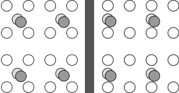
There are two commonly used chroma siting patterns, as illustrated by the graphic above. Most digital video today uses the MPEG-2 variant, that is, left-aligned chroma. This is essential to keep in mind when going from 4:2:0 to 4:4:4, because if the chroma planes are naively upscaled and joined with the luma plane without any shifting, the chroma will be shifted by a quarter pixel. This is a consequence of the way output pixels are usually mapped onto the input grid during resampling:
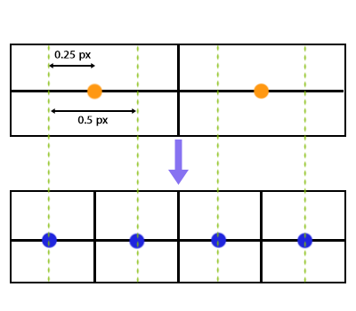
Essentially, the output grid is scaled such that the outer edges of the pixel boxes align, importantly under the assumption that samples are center-aligned within the pixel boxes. Therefore, when scaling a chroma plane by 200%, which is what happens to the chroma when going from 4:2:0 to 4:4:4, the new chroma sample positions will match up with the luma sample positions. This would be the correct mapping if the resamplers’s assumption of center-alignment was true—if it isn’t (like with MPEG-2 chroma placement) we have to compensate for the offset by shifting the input samples by a quarter pixel width to the left before calculating the output samples. This way, the left-alignment is restored.
This quarter-pixel shifting is performed automatically under the hood by most format conversion software and media players. Thus, we only need to take care of it if we handle the chroma upscaling separately by hand.
In VS,
shifting can be performed with the resize functions’ src_left parameter:
u = core.std.ShufflePlanes(src, planes=1, colorfamily=vs.GRAY)
shifted_scaled_u = core.resize.Spline16(u, 1920, 1080, src_left=0.25) # shifts the image to the left by 0.25 pixels
-
The Fourier transform is an ubiquitous concept in image processing, so we strongly advise becoming familiar with at least the basics. A very good resource for this topic is ImageMagick’s guide. ↩
-
Robidoux, N. (2012, October 21). Resampling — ImageMagick v6 Examples. Retrieved August 22, 2019, from https://www.imagemagick.org/Usage/filter/nicolas/#upsampling ↩
-
If you don’t understand what this means, read the resources linked above in the resizing section. ↩